Books: 2011-02-06

Wednesday 9 February 2011

Data Files (Matlab tutorial)

Data Files

Matlab does not allow you to save the commands that you have entered in a session, but it does allow a number of different ways to save the data. In this tutorial we explore the different ways that you can save and read data into a Matlab session.

Saving and Recalling Data
Saving a Session as Text
C Style Read/Write

Saving and Recalling Data

As you work through a session you generate vectors and matrices. The next question is how do you save your work? Here we focus on how to save and recall data from a Matlab session. The command to save all of the data in a session is save. The command to bring the data set in a data file back into a session isload.
We first look at the save command. In the example below we use the most basic form which will save all of the data present in a session. Here we save all of the data in a file called "stuff.mat." (.mat is the default extension for Matlab data.)

>> u = [1 3 -4];
 >> v = [2 -1 7];
 >> whos
   Name      Size                    Bytes  Class

   u         1x3                        24  double array
   v         1x3                        24  double array

 Grand total is 6 elements using 48 bytes

 >> save stuff.mat
 >> ls
 stuff.mat

The ls command is used to list all of the files in the current directory. In this situation we created a file called "stuff.mat" which contains the vectors u and v. The data can be read back in to a Matlab session with the load command.

>> clear
 >> whos
 >> load stuff.mat
 >> whos
   Name      Size                    Bytes  Class

   u         1x3                        24  double array
   v         1x3                        24  double array

 Grand total is 6 elements using 48 bytes

 >> u+v

 ans =

      3     2     3

In this example the current data space is cleared of all variables. The contents of the entire data file, "stuff.mat," is then read back into memory. You do not have to load all of the contents of the file into memory. After you specify the file name you then list the variables that you want to load separated by spaces. In the following example only the variable u will be loaded into memory.

>> clear
 >> whos
 >> load stuff.mat u
 >> whos
   Name      Size                    Bytes  Class

   u         1x3                        24  double array

 Grand total is 3 elements using 24 bytes

 >> u

 u =

      1     3    -4

Note that the save command works in exactly the same way. If you only want to save a couple of variables you list the variables you want to save after the file name. Again, the variables must be separated by a space. For an example and more details please see the help file for save. When in matlab just type in help save to see more information. You will find that there are large number of options in terms of how the data can be saved and the format of the data file.

Saving a Session as Text

Matlab allows you to save the data generated in a session, but you cannot easily save the commands so that they can be used in an executable file. You can save a copy of what happened in a session using the diary command. This is very useful if you want to save a session for a homework assignment or as a way to take notes.
A diary of a session is initiated with the diary command followed by the file name that you want to keep the text file. You then type in all of the necessary commands. When you are done enter the diary command alone, and it will write all of the output to the file and close the file. In the example below a file called "save.txt" is created that will contain a copy of the session.

>> diary save.txt
  ... enter commands here...
 >> diary

This will create a file called "save.txt" which will hold an exact copy of the output from your session. This is how I generated the files used in these tutorials.

C Style Read/Write

In addition to the high level read/write commands detailed above, Matlab allows C style file access. This is extremely helpful since the output generated by many home grown programs is in binary format due to disk space considerations. This is an advanced subject, and we do not go into great detail here. Instead we look at the basic commands. After looking at this overview we highly recommend that you look through the relevant help files. This will help fill in the missing blanks.
The basic idea is that you open a file, execute the relevant reads and writes on a file, and then close a file. One other common task is to move the file pointer to point to a particular place in the file, and there are two commands, fseek and ftell to help.
Here we give a very simple example. In the example, a file called "laser.dat" is opened. The file identifier is kept track of using a variable called fp. Once the file is opened the file position is moved to a particular place in the file, denoted pos, and two double precision numbers are read. Once that is done the position within the file is stored, and the file is closed.

fp = fopen('laser.dat','r');
 fseek(fp,pos,'bof');
 tmp = fread(fp,2,'double');
 pos = ftell(fp);
 fclose(fp);

The If Statement(matlab tutorial)

The If Statement

In this tutorial we will assume that you know how to create vectors and matrices, know how to index into them, and know about loops. For more information on those topics see one of our tutorials on vectors, matrices, vector operations, loops, plotting, executable files, or subroutines.
There are times when you want your code to make a decision. For example, if you are approximating a differential equation, and the rate of change is discontinuous, you may want to change the rate depending on what time step you are on.
Here we will define an executable file that contains an if statement. The file is called by Matlab, and it constructs a second derivative finite difference matrix with boundary conditions. There is a variable in the file called decision. If this variable is less than 3, the file will find and plot the eigen values of the matrix, if it is greater than 3 the eigen values of the inverse of the matrix are found and plotted, otherwise, the system is inverted to find an approximation to y'=sin(x) according to the specified boundary conditions.

There are times when you want certain parts of your program to be executed only in limited circumstances. The way to do that is to put the code within an "if" statement. The most basic structure for an "if" statement is the following:

if  (condition statement)
    (matlab commands)
end

More complicated structures are also possible including combinations like the following:

if  (condition statement)
    (matlab commands)
elseif  (condition statement)
    (matlab commands)
elseif (condition statement)
    (matlab commands)
.
.
.
else
    (matlab commands)
end

The conditions are boolean statements and the standard comparisons can be made. Valid comparisons include "<" (less than), ">" (greater than), "<=" (less than or equal), ">=" (greater than or equal), "==" (equal - this is two equal signs with no spaces betweeen them), and "˜=" (not equal). For example, the following code will set the variable j to be -1:

a = 2;
b = 3;
if (a<b) 
    j = -1;
end

Additional statements can be added for more refined decision making. The following code sets the variable j to be 2.

a = 4;
b = 3;
if (a<b) 
    j = -1;
elseif (a>b)
    j = 2;
end

The else statement provides a catch all that will be executed if no other condition is met. The following code sets the variable j to be 3.

a = 4;
b = 4;
if (a<b) 
    j = -1;
elseif (a>b)
    j = 2;
else 
 j = 3
end

This last example demonstrates one of the bad habits that Matlab allows you to get away with. With finite precision arithmetic two variables are rarely exactly the same. When using C or FORTRAN you should never compare two floating numbers to see if they are the same. Instead you should check to see if they are close. Matlab does not use integer arithmetic so if you check to see if two numbers are the same it automatically checks to see if the variables are close. If you were to use C or FORTRAN then that last example could get you into big trouble. but Matlab does the checking for you in case the numbers are just really close.

Matlab allows you to string together multiple boolean expressions using the standard logic operators, "&" (and), ¦ (or), and ˜ (not). For example to check to see if a is less than b and at the same time b is greater than or equal to c you would use the following commands:

if (a < b) & (b >= c) 
   Matlab commands
end

Example

If you are not familiar with creating exectable files see our tutorial on the subject. Otherwise, copy the following script into a file called ifDemo.m.

decision = 3;
leftx = 0;
rightx = 1;

lefty = 1;
righty = 1;

N= 10;
h = (rightx-leftx)/(N-1);
x = [leftx:h:rightx]';

A = zeros(N);

for i=2:N-1,
   A(i,i-1:i+1) = [1 -2 1];
end

A = A/h^2;

A(1,1) = 1;
A(N,N) = 1;

b = sin(x);
b(1) = lefty;
b(N) = righty;

if(decision<3)

    % Find and plot the eigen values
    [e,v] = eig(A);
    e = diag(e);
    plot(real(e),imag(e),'rx');
    title('Eigen Values of the matrix');

elseif(decision>3)

    % Find and plot the eigen values of inv(A)
    [e,v] = eig(inv(A));
    e = diag(e);
    plot(real(e),imag(e),'rx');
    title('Eigen Values of the inverse of the matrix');

else

   
    % Solve the system
    y = A\b;
    linear = (lefty-righty+sin(leftx)-sin(rightx))/(leftx-rightx);
    constant = lefty + sin(leftx) - linear*leftx;
    true = -sin(x) + linear*x + constant;

    subplot(1,2,1);
    plot(x,y,'go',x,true,'y');
    title('True Solution and Approximation');
    xlabel('x');
    ylabel('y');
    subplot(1,2,2);
    plot(x,abs(y-true),'cx');
    title('Error');
    xlabel('x');
    ylabel('|Error|');


end

You can execute the instructions in the file by simply typing ifDemo at the matlab prompt. Try changing the value of the variable decision to see what actions the script will take. Also, try changing the other variables and experiment.
The basic form of the if-block is demonstrated in the program above. You are not required to have an elseif or else block, but you are required to end the if-block with the endif statement.

Subroutines in matlab

Subroutines

In this tutorial we will assume that you know how to create vectors and matrices, know how to index into them, and know about loops. For more information on those topics see one of our tutorials on vectors, matrices, vector operations, loops, plotting, or executable files.
Sometimes you want to repeat a sequence of commands, but you want to be able to do so with different vectors and matrices. One way to make this easier is through the use of subroutines. Subroutines are just like executable files, but you can pass it different vectors and matrices to use.
For example, suppose you want a subroutine to perform Gaussian elimination, and you want to be able to pass the matrix and pass the vector (This example comes from the tutorial on loops). The first line in the file has to tell matlab what variables it will pass back when and done, and what variables it needs to work with. Here we will try to find x given that Ax=b.
The routine needs the matrix A and the vector B, and it will pass back the vector x. If the name of the file is called gaussElim.m, then the first line will look like this:
function [x] = gaussElim(A,b)
If you want to pass back more than one variable, you can include the list in the brackets with commas in between the variable names (see the second example). If you do not know how to create a file see our tutorial on executable files.

Here is a sample listing of the file gaussElim.m:

function [x] = gaussElim(A,b)
% File gaussElim.m
%   This subroutine will perform Gaussian elmination
%   on the matrix that you pass to it.
%   i.e., given A and b it can be used to find x,
%        Ax = b
%
%   To run this file you will need to specify several
%   things:
%   A - matrix for the left hand side.
%   b - vector for the right hand side
%
%   The routine will return the vector x.
%   ex: [x] = gaussElim(A,b)
%     this will perform Gaussian elminiation to find x.
%
%


 N = max(size(A));


% Perform Gaussian Elimination

 for j=2:N,
     for i=j:N,
        m = A(i,j-1)/A(j-1,j-1);
        A(i,:) = A(i,:) - A(j-1,:)*m;
        b(i) = b(i) - m*b(j-1);
     end
 end

% Perform back substitution

 x = zeros(N,1);
 x(N) = b(N)/A(N,N);

 for j=N-1:-1:1,
   x(j) = (b(j)-A(j,j+1:N)*x(j+1:N))/A(j,j);
 end

To get the vector x, you simply call the routine by name. For example, you could do the following:

>> A = [1 2 3 6; 4 3 2 3; 9 9 1 -2; 4 2 2 1]

A =

     1     2     3     6
     4     3     2     3
     9     9     1    -2
     4     2     2     1

>> b = [1 2 1 4]'

b =

     1
     2
     1
     4

>> [x] = gaussElim(A,b)


x =

    0.6809
   -0.8936
    1.8085
   -0.5532

>>

Sometimes you want your routine to call another routine that you specify. For example, here we will demonstrate a subroutine that will approximate a D.E., y'=f(x,y), using Euler's Method. The subroutine is able to call a function, f(x,y), specified by you.
Here a subroutine is defined that will approximate a D.E. using Euler's method. If you do not know how to create a file see our tutorial on executable files.

Here is a sample listing of the file eulerApprox.m:

function [x,y] = eulerApprox(startx,h,endx,starty,func)
% file: eulerApprox.m
% This matlab subroutine will find the approximation to
%  a D.E. given by 
%     y' = func(x,y)
%     y(startx) = starty
%
%  To run this file you will first need to specify
%  the following:
%      startx  : the starting value for x
%      h       : the step size
%      endx    : the ending value for x
%      starty  : the initial value
%      func    : routine name to calculate the right hand 
%                side of the D.E..  This must be specified
%                as a string.
%
%   ex: [x,y] = eulerApprox(0,1,1/16,1,'f');
%       Will return the approximation of a D.E.
%       where x is from 0 to 1 in steps of 1/16.
%       The initial value is 1, and the right hand
%       side is calculated in a subroutine given by
%       f.m.
%
%  The routine will generate two vectors.  The first
%  vector is x which is the grid points starting at
%  x0=0 and have a step size h.  
%
%  The second vector is an approximation to the specified
%  D.E. 
%



x = [startx:h:endx];

y = 0*x;
y(1) = starty;

for i=2:max(size(y)),
   y(i) = y(i-1) + h*feval(func,x(i-1),y(i-1));
end

In this example, we will approximate the D.E. y'=1/y. To do this you will have to create a file called f.m with the following commands:

function [f] = f(x,y)
% Evaluation of right hand side of a differential
% equation.  

f = 1/y;

With the subroutine defined, you can call it whenever necessary. Note that when you put comments on the 2nd line, it acts as a help file. Also note that the function f.m must be specified as a string, 'f'.

>> help eulerApprox

  file: eulerApprox.m
  This matlab subroutine will find the approximation to
   a D.E. given by 
      y' = func(x,y)
      y(startx) = starty
 
   To run this file you will first need to specify
   the following:
       startx  : the starting value for x
       h       : the step size
       endx    : the ending value for x
       starty  : the initial value
       func    : routine name to calculate the right hand 
                 side of the D.E..  This must be specified
                 as a string.
 
    ex: [x,y] = eulerApprox(0,1,1/16,1,'f');
        Will return the approximation of a D.E.
        where x is from 0 to 1 in steps of 1/16.
        The initial value is 1, and the right hand
        side is calculated in a subroutine given by
        f.m.
 
   The routine will generate two vectors.  The first
   vector is x which is the grid points starting at
   x0=0 and have a step size h.  
 
   The second vector is an approximation to the specified
   D.E. 
 

>> [x,y] = eulerApprox(0,1/16,1,1,'f');
>> plot(x,y)

When the subroutine is done, it returns two vectors and stores them in x and y.

Executable Files

In this tutorial we will assume that you know how to create vectors and matrices, know how to index into them, and know about loops. For more information on those topics see one of our tutorials on vectors, matrices, vector operations, loops, or plotting.
In this tutorial we will introduce the basic operations for creating executable files. Once you have a general routine in a matlab file, it allows you to perform more complex operations, and it is easier to repeat these operations. For example, you might have a set of instructions to use Euler's approximation for a differential equation (see the tutorial on loops), but you want to be able to use those instructions for different equations.
As an example, a simple file to approximate the D.E. y'= 1/y using Euler's method is found. To execute the commands in the file, the step size and the initial value must be specified. Once done, you can easily approximate the given D.E. for a wide variey of initial conditions and step sizes.
First, you will need to create the file. The easiest editor on our system is to just use the built in matlab editor. It will allow you to do some very simple file manipulations. The editor is very simple and easy to start. It is not a very advanced editor, though.
Matlab executable files (called M-files) must have the extension ".m". In this example a file called simpleEuler.m is created. To get Matlab to execute the commands in the file simply type in "simpleEuler". Matlab will then search the current directory for the file "simpleEuler", read the file, and execute the commands in the file. If matlab cannot find the file you will get an error message:
??? Undefined function or variable 'simpleEuler'.
If this is the case then either you mistyped the name of the program, the program is misnamed, or the file is located in directory that matlab does not know about. In the later case you have to let matlab know which directory to search. The list of directories that is searched for files is called the "path." For more information on how to set the path there are two articles at the mathworks site that go into more detail: text command and graphical.
If you are not familiar with a more advanced editor use matlab's built in editor to create the file. Type in the following command at the matlab prompt:

>> edit simpleEuler.m

Once the editor appears on the screen either type or cut and paste the necessary matlab commands:

% file: simpleEuler.m
% This matlab file will find the approximation to
%
% dy/dx =  1/y
% y(0) = starty
%
%
%  To run this file you will first need to specify
%  the step the following:
%      h       : the step size
%      starty  : the initial value
%
%  The routine will generate three vectors.  The first
%  vector is x which is the grid points starting at
%  x0=0 and have a step size h.  
%
%  The second vector is an approximation to the specified
%  D.E. 
%
%  The third vector is the true solution to the D.E.
%
%  If you haven't guessed, you cna use the percent sign
%  to add comments.
%



x = [0:h:1];

y = 0*x;
y(1) = starty;

for i=2:max(size(y)),
   y(i) = y(i-1) + h/y(i-1);
end

true = sqrt(2*x+1);

Once the commands are in place, save the file. Go back to your original window and start up matlab. The file is called up by simply typing in the base name (in this case simpleEuler).

>> simpleEuler
??? Undefined function or variable h.

Error in ==> /home/black/math/mat/examples/simpleEuler.m
On line 28  ==> x = [0:h:1];

If you try to call the file without first defining the variables h and starty, you will get an error message. You must first specify all of the variables that are not defined in the file itself.

>> h = 1/16;
>> starty = 1;
>> simpleEuler
>> whos
  Name         Size                   Bytes  Class

  h            1x1                        8  double array
  i            1x1                        8  double array
  starty       1x1                        8  double array
  true         1x17                     136  double array
  x            1x17                     136  double array
  y            1x17                     136  double array

Grand total is 54 elements using 432 bytes

>> plot(x,y,'rx',x,true)

Once the necessary variables are defined, and you type in the command simpleEuler, matlab searched the current directory for a file called simpleEuler.m. Once it found the file, it read the file and executed the commands as if you had typed them from the keyboard.
If you would like to run the program again with a different step size, you have to be careful. The program will write over the vectors x,y, and true. If you want to save these vectors, you must do so explicitly!

>> x0 = x;
>> y0 = y;
>> true0 = true;
>> h = h/2;
>> simpleEuler
>> whos
  Name         Size                   Bytes  Class

  h            1x1                        8  double array
  i            1x1                        8  double array
  starty       1x1                        8  double array
  true         1x33                     264  double array
  true0        1x17                     136  double array
  x            1x33                     264  double array
  x0           1x17                     136  double array
  y            1x33                     264  double array
  y0           1x17                     136  double array

Grand total is 153 elements using 1224 bytes

>> plot(x0,abs(true0-y0),'gx',x,abs(true-y),'yo');

Now you have two approximations. The first is with a step size of 1/16, and it is stored in the vectors x0 and y0. The second approximation is for a step size of 1/32 and is found in the vectorsx and y.

Plotting

>> h = 1/16;
>> x = 0:h:1;
>> y = 0*x;
>> size(y)

ans =

     1    17

>> max(size(y))

ans =

    17

>> y(1) = 1;
>> for i=2:max(size(y)),
     y(i) = y(i-1) + h/y(i-1);
   end
>> true = sqrt(2*x+1);

Now, we have an approximation and the true solution. To compare the two, the true solution is plotted with the approximation plotted at the grid points as a green 'o'. The plot command is used to generate plots in matlab. There is a wide variety of arguments that it will accept. Here we just want one plot, so we give it the range, the domain, and the format.

>> plot(x,y,'go',x,true)

That's nice, but it would also be nice to plot the error:

>> plot(x,abs(true-y),'mx')

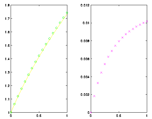
Okay, let's print everything on one plot. To do this, you have to tell matlab that you want two plots in the picture. This is done with the subplot command. Matlab can treat the window as an array of plots. Here we will have one row and two columns giving us two plots. In plot #1 the function is plotted, while in plot #2 the error is plotted.

>> subplot(1,2,1);
>> plot(x,y,'go',x,true)
>> subplot(1,2,2);
>> plot(x,abs(true-y),'mx')

Figure 1. The two plots from the first approximation

Let's start over. A new approximation is found by cutting the step size in half. But first, the picture is completely cleared and reset using the clf comand. (Note that I am using new vectors x1and y1.)

>> clf
>> h = h/2;
>> x1 = 0:h:1;
>> y1 = 0*x1;
>> y1(1) = 1;
>> for i=2:max(size(y1)),
     y1(i) = y1(i-1) + h/y1(i-1);
   end
>> true1 = sqrt(2*x1+1);

The new approximation is plotted, but be careful! The vectors passed to plot have to match. The labels are given for the axis and a title is given to each plot in the following example. The following example was chosen to show how you can use the subplot command to cycle through the plots at any time.

>> plot(x,y1,'go',x,true1)
??? Error using ==> plot
Vectors must be the same lengths.

>> plot(x1,y1,'go',x1,true1)
>> plot(x1,abs(true1-y1),'mx')
>> subplot(1,2,1);
>> plot(x,abs(true-y),'mx')
>> subplot(1,2,2);
>> plot(x1,abs(true1-y1),'mx')
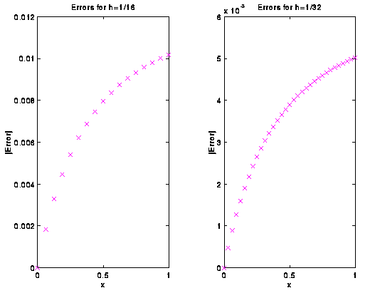
>> title('Errors for h=1/32')
>> xlabel('x');
>> ylabel('|Error|');
>> subplot(1,2,1);
>> xlabel('x');
>> ylabel('|Error|');
>> title('Errors for h=1/16')

Figure 2. The errors for the two approximations

Finally, if you want to print the plot, you must first print the plot to a file. To print a postscript file of the current plot you can use the print command. The following example creates a postscript file called error.ps which resides in the current directory. This new file (error.ps) can be printed from the UNIX prompt using the lpr command.

>> print -dps error.ps

Loops in matlab

Loops

In this tutorial we will demonstrate how the for and the while loop are used. First, the for loop is discussed with examples for row operations on matrices and for Euler's Method to approximate an ODE. Following the for loop, a demonstration of the while loop is given.
We will assume that you know how to create vectors and matrices and know how to index into them. For more information on those topics see one of our tutorials on either vectors, matrices, or vector operations.

For Loops
While Loops

For Loops

The for loop allows us to repeat certain commands. If you want to repeat some action in a predetermined way, you can use the for loop. All of the loop structures in matlab are started with a keyword such as "for", or "while" and they all end with the word "end". Another deep thought, eh.
The for loop is written around some set of statements, and you must tell Matlab where to start and where to end. Basically, you give a vector in the "for" statement, and Matlab will loop through for each value in the vector:
For example, a simple loop will go around four times each time changing a loop variable, j:

>> for j=1:4,
   j
end


j =

     1


j =

     2


j =

     3


j =

     4

>>

When Matlab reads the "for" statement it constructs a vector, [1:4], and j will take on each value within the vector in order. Once Matlab reads the "end" statement, it will execute and repeat the loop. Each time the for statement will update the value of j and repeat the statements within the loop. In this example it will print out the value of j each time.
For another example, we define a vector and later change the entries. Here we step though and change each individual entry:

>> v = [1:3:10]

v =

     1     4     7    10

>> for j=1:4,
     v(j) = j;
end
>> v

v =

     1     2     3     4

Note, that this is a simple example and is a nice demonstration to show you how a for loop works. However, DO NOT DO THIS IN PRACTICE!!!! Matlab is an interpreted language and looping through a vector like this is the slowest possible way to change a vector. The notation used in the first statement is much faster than the loop.
A better example, is one in which we want to perform operations on the rows of a matrix. If you want to start at the second row of a matrix and subtract the previous row of the matrix and then repeat this operation on the following rows, a for loop can do this in short order:

>> A = [ [1 2 3]' [3 2 1]' [2 1 3]']

A =

     1     3     2
     2     2     1
     3     1     3

>> B = A;
>> for j=2:3,
    A(j,:) = A(j,:) - A(j-1,:)
end

A =

     1     3     2
     1    -1    -1
     3     1     3


A =

     1     3     2
     1    -1    -1
     2     2     4

For a more realistic example, since we can now use loops and perform row operations on a matrix, Gaussian Elimination can be performed using only two loops and one statement:

>> for j=2:3,
     for i=j:3,
        B(i,:) = B(i,:) - B(j-1,:)*B(i,j-1)/B(j-1,j-1)
     end
   end

B =

     1     3     2
     0    -4    -3
     3     1     3


B =

     1     3     2
     0    -4    -3
     0    -8    -3


B =

     1     3     2
     0    -4    -3
     0     0     3

Another example where loops come in handy is the approximation of differential equations. The following example approximates the D.E. y'=x^2-y^2, y(0)=1, using Euler's Method. First, the step size, h, is defined. Once done, the grid points are found, and an approximation is found. The approximation is simply a vector, y, in which the entry y(j) is the approximation at x(j).

>> h = 0.1;
>> x = [0:h:2];
>> y = 0*x;
>> y(1) = 1;
>> size(x)

ans =

     1    21

>> for i=2:21,
    y(i) = y(i-1) + h*(x(i-1)^2 - y(i-1)^2);
   end
>> plot(x,y)
>> plot(x,y,'go')
>> plot(x,y,'go',x,y)

While Loops

If you don't like the for loop, you can also use a while loop. The while loop repeats a sequence of commands as long as some condition is met. This can make for a more efficient algorithm. In the previous example the number of time steps to make may be much larger than 20. In such a case the for loop can use up a lot of memory just creating the vector used for the index. A better way of implementing the algorithm is to repeat the same operations but only as long as the number of steps taken is below some threshold. In this example the D.E. y'=x-|y|, y(0)=1, is approximated using Euler's Method:

>> h = 0.001;
>> x = [0:h:2];
>> y = 0*x;
>> y(1) = 1;
>> i = 1;
>> size(x)

ans =

           1        2001

>> max(size(x))

ans =

        2001

>> while(i<max(size(x)))
     y(i+1) = y(i) + h*(x(i)-abs(y(i)));
     i = i + 1;                         
   end
>> plot(x,y,'go')
>> plot(x,y)

Vector Functions

Matlab makes it easy to create vectors and matrices. The real power of Matlab is the ease in which you can manipulate your vectors and matrices. Here we assume that you know the basics of defining and manipulating vectors and matrices. In particular we assume that you know how to create vectors and matrices and know how to index into them. For more information on those topics see our tutorial on either vectors or matrices.
In this tutorial we will first demonstrate simple manipulations such as addition, subtraction, and multiplication. Following this basic "element-wise" operations are discussed. Once these operations are shown, they are put together to demonstrate how relatively complex operations can be defined with little effort.
First, we will look at simple addition and subtraction of vectors. The notation is the same as found in most linear algebra texts. We will define two vectors and add and subtract them:

>> v = [1 2 3]'

v =

     1
     2
     3

>> b = [2 4 6]'

b =

     2
     4
     6

>> v+b

ans =

     3
     6
     9

>> v-b

ans =

    -1
    -2
    -3

Multiplication of vectors and matrices must follow strict rules. Actually, so must addition. In the example above, the vectors are both column vectors with three entries. You cannot add a row vector to a column vector. Multiplication, though, can be a bit trickier. The number of columns of the thing on the left must be equal to the number of rows of the thing on the right of the multiplication symbol:

>> v*b 
??? Error using ==> *
Inner matrix dimensions must agree.

>> v*b'

ans =

     2     4     6
     4     8    12
     6    12    18

>> v'*b

ans =

    28

There are many times where we want to do an operation to every entry in a vector or matrix. Matlab will allow you to do this with "element-wise" operations. For example, suppose you want to multiply each entry in vector v with its cooresponding entry in vector b. In other words, suppose you want to find v(1)*b(1), v(2)*b(2), and v(3)*b(3). It would be nice to use the "*" symbol since you are doing some sort of multiplication, but since it already has a definition, we have to come up with something else. The programmers who came up with Matlab decided to use the symbols ".*" to do this. In fact, you can put a period in front of any math symbol to tell Matlab that you want the operation to take place on each entry of the vector.

>> v.*b

ans =

     2
     8
    18

>> v./b

ans =

    0.5000
    0.5000
    0.5000

Since we have opened the door to non-linear operations, why not go all the way? If you pass a vector to a predefined math function, it will return a vector of the same size, and each entry is found by performing the specified operation on the cooresponding entry of the original vector:

>> sin(v)

ans =

    0.8415
    0.9093
    0.1411

>> log(v)

ans =

         0
    0.6931
    1.0986

The ability to work with these vector functions is one of the advantages of Matlab. Now complex operations can be defined that can be done quickly and easily. In the following example a very large vector is defined and can be easily manipulated. (Notice that the second command has a ";" at the end of the line. This tells Matlab that it should not print out the result.)

>> x = [0:0.1:100]

x =

  Columns 1 through 7 

         0    0.1000    0.2000    0.3000    0.4000    0.5000    0.6000

    [stuff deleted]

  Columns 995 through 1001 

   99.4000   99.5000   99.6000   99.7000   99.8000   99.9000  100.0000


>> y = sin(x).*x./(1+cos(x));

Through this simple manipulation of vectors, Matlab will also let you graph the results. The following example also demonstrates one of the most useful commands in Matlab, the "help" command.

>> plot(x,y)
>> plot(x,y,'rx')
>> help plot

 PLOT   Linear plot. 
    PLOT(X,Y) plots vector Y versus vector X. If X or Y is a matrix,
    then the vector is plotted versus the rows or columns of the matrix,
    whichever line up.  If X is a scalar and Y is a vector, length(Y)
    disconnected points are plotted.
 
    PLOT(Y) plots the columns of Y versus their index.
    If Y is complex, PLOT(Y) is equivalent to PLOT(real(Y),imag(Y)).
    In all other uses of PLOT, the imaginary part is ignored.
 
    Various line types, plot symbols and colors may be obtained with
    PLOT(X,Y,S) where S is a character string made from one element
    from any or all the following 3 columns:
 
           b     blue          .     point              -     solid
           g     green         o     circle             :     dotted
           r     red           x     x-mark             -.    dashdot 
           c     cyan          +     plus               --    dashed   
           m     magenta       *     star
           y     yellow        s     square
           k     black         d     diamond
                               v     triangle (down)
                               ^     triangle (up)
                               <     triangle (left)
                               >     triangle (right)
                               p     pentagram
                               h     hexagram
                          
    For example, PLOT(X,Y,'c+:') plots a cyan dotted line with a plus 
    at each data point; PLOT(X,Y,'bd') plots blue diamond at each data 
    point but does not draw any line.
 
    PLOT(X1,Y1,S1,X2,Y2,S2,X3,Y3,S3,...) combines the plots defined by
    the (X,Y,S) triples, where the X's and Y's are vectors or matrices 
    and the S's are strings.  
 
    For example, PLOT(X,Y,'y-',X,Y,'go') plots the data twice, with a
    solid yellow line interpolating green circles at the data points.
 
    The PLOT command, if no color is specified, makes automatic use of
    the colors specified by the axes ColorOrder property.  The default
    ColorOrder is listed in the table above for color systems where the
    default is blue for one line, and for multiple lines, to cycle
    through the first six colors in the table.  For monochrome systems,
    PLOT cycles over the axes LineStyleOrder property.
 
    PLOT returns a column vector of handles to LINE objects, one
    handle per line. 
 
    The X,Y pairs, or X,Y,S triples, can be followed by 
    parameter/value pairs to specify additional properties 
    of the lines.
                                    
    See also SEMILOGX, SEMILOGY, LOGLOG, PLOTYY, GRID, CLF, CLC, TITLE,
    XLABEL, YLABEL, AXIS, AXES, HOLD, COLORDEF, LEGEND, SUBPLOT, STEM.

 Overloaded methods
    help idmodel/plot.m
    help iddata/plot.m


>> plot(x,y,'y',x,y,'go')
>> plot(x,y,'y',x,y,'go',x,exp(x+1),'m--')
>> whos
  Name      Size                   Bytes  Class

  ans       3x1                       24  double array
  b         3x1                       24  double array
  v         3x1                       24  double array
  x         1x1001                  8008  double array
  y         1x1001                  8008  double array

Grand total is 2011 elements using 16088 bytes

The compact notation will let you tell the computer to do lots of calculations using few commands. For example, suppose you want to calculate the divided differences for a given equation. Once you have the grid points and the values of the function at those grid points, building a divided difference table is simple:

>> coef = zeros(1,1001);
>> coef(1) = y(1);
>> y = (y(2:1001)-y(1:1000))./(x(2:1001)-x(1:1000));
>> whos
  Name       Size                   Bytes  Class

  ans        3x1                       24  double array
  b          3x1                       24  double array
  coef       1x1001                  8008  double array
  v          3x1                       24  double array
  x          1x1001                  8008  double array
  y          1x1000                  8000  double array

Grand total is 3008 elements using 24064 bytes

>> coef(2) = y(1);
>> y(1)

ans =

    0.0500

>> y = (y(2:1000)-y(1:999))./(x(3:1001)-x(1:999));
>> coef(3) = y(1);
>> 
>>

From this algorithm you can find the Lagrange polynomial that interpolates the points you defined above (vector x). Of course, with so many points, this might get a bit tedious. Fortunately, matlab has an easy way of letting the computer do the repetitive things, which is examined in the next tutorial.

Introduction to Matrices in Matlab

A basic introduction to defining and manipulating matrices is given here. It is assumed that you know the basics on how to define and manipulate vectors using matlab.

Defining Matrices
Matrix Functions
Matrix Operations

Defining Matrices

Defining a matrix is similar to defining a vector. To define a matrix, you can treat it like a column of row vectors (note that the spaces are required!):

>> A = [ 1 2 3; 3 4 5; 6 7 8]

A =

     1     2     3
     3     4     5
     6     7     8

You can also treat it like a row of column vectors:

>> B = [ [1 2 3]' [2 4 7]' [3 5 8]']

B =

     1     2     3
     2     4     5
     3     7     8

(Again, it is important to include the spaces.)
If you have been putting in variables through this and the tutorial on vectors, then you probably have a lot of variables defined. If you lose track of what variables you have defined, the whos command will let you know all of the variables you have in your work space.

>> whos
  Name      Size                   Bytes  Class

  A         3x3                       72  double array
  B         3x3                       72  double array
  v         1x5                       40  double array

Grand total is 23 elements using 184 bytes

We assume that you are doing this tutorial after completing the previous tutorial. The vector v was defined in the previous tutorial.
As mentioned before, the notation used by Matlab is the standard linear algebra notation you should have seen before. Matrix-vector multiplication can be easily done. You have to be careful, though, your matrices and vectors have to have the right size!

>> v = [0:2:8]

v =

     0     2     4     6     8

>> A*v(1:3)
??? Error using ==> *
Inner matrix dimensions must agree.

>> A*v(1:3)'

ans =

    16
    28
    46

Get used to seeing that particular error message! Once you start throwing matrices and vectors around, it is easy to forget the sizes of the things you have created.
You can work with different parts of a matrix, just as you can with vectors. Again, you have to be careful to make sure that the operation is legal.

>> A(1:2,3:4)
???  Index exceeds matrix dimensions.

>> A(1:2,2:3)

ans =

     2     3
     4     5

>> A(1:2,2:3)'

ans =

     2     4
     3     5

Matrix Functions

Once you are able to create and manipulate a matrix, you can perform many standard operations on it. For example, you can find the inverse of a matrix. You must be careful, however, since the operations are numerical manipulations done on digital computers. In the example, the matrix A is not a full matrix, but matlab's inverse routine will still return a matrix.

>> inv(A)

Warning: Matrix is close to singular or badly scaled.
         Results may be inaccurate. RCOND = 4.565062e-18


ans =

   1.0e+15 *

   -2.7022    4.5036   -1.8014
    5.4043   -9.0072    3.6029
   -2.7022    4.5036   -1.8014

By the way, Matlab is case sensitive. This is another potential source of problems when you start building complicated algorithms.

>> inv(a)
??? Undefined function or variable a.

Other operations include finding an approximation to the eigen values of a matrix. There are two versions of this routine, one just finds the eigen values, the other finds both the eigen values and the eigen vectors. If you forget which one is which, you can get more information by typing help eig at the matlab prompt.

>> eig(A)

ans =

   14.0664
   -1.0664
    0.0000

>> [v,e] = eig(A)

v =

   -0.2656    0.7444   -0.4082
   -0.4912    0.1907    0.8165
   -0.8295   -0.6399   -0.4082


e =

   14.0664         0         0
         0   -1.0664         0
         0         0    0.0000

>> diag(e)

ans =

   14.0664
   -1.0664
    0.0000

Matrix Operations

There are also routines that let you find solutions to equations. For example, if Ax=b and you want to find x, a slow way to find x is to simply invert A and perform a left multiply on both sides (more on that later). It turns out that there are more efficient and more stable methods to do this (L/U decomposition with pivoting, for example). Matlab has special commands that will do this for you.
Before finding the approximations to linear systems, it is important to remember that if A and B are both matrices, then AB is not necessarily equal to BA. To distinguish the difference between solving systems that have a right or left multiply, Matlab uses two different operators, "/" and "\". Examples of their use are given below. It is left as an exercise for you to figure out which one is doing what.

>> v = [1 3 5]'

v =

     1
     3
     5

>> x = A\v

Warning: Matrix is close to singular or badly scaled.
         Results may be inaccurate. RCOND = 4.565062e-18


x =

   1.0e+15 *

    1.8014
   -3.6029
    1.8014

>> x = B\v

x =

     2
     1
    -1

>> B*x

ans =

     1
     3
     5

>> x1 = v'/B

x1 =

    4.0000   -3.0000    1.0000


>> x1*B

ans =

    1.0000    3.0000    5.0000

Finally, sometimes you would like to clear all of your data and start over. You do this with the "clear" command. Be careful though, it does not ask you for a second opinion and its results arefinal.

>> clear

>> whos

Introduction to Vectors in Matlab

This is the basic introduction to Matlab. Creation of vectors is included with a few basic operations. Topics include the following:

Defining a Vector

Matlab is a software package that makes it easier for you to enter matrices and vectors, and manipulate them. The interface follows a language that is designed to look a lot like the notation use in linear algebra. In the following tutorial, we will discuss some of the basics of working with vectors.
If you are running windows or Mac OSX, you can start matlab by choosing it from the menu. To start matlab on a unix system, open up a unix shell and type the command to start the software: matlab. This will start up the software, and it will wait for you to enter your commands. In the text that follows, any line that starts with two greater than signs (>>) is used to denote the matlab command line. This is where you enter your commands.
Almost all of Matlab's basic commands revolve around the use of vectors. A vector is defined by placing a sequence of numbers within square braces:

>> v = [3 1]

v =

     3     1

This creates a row vector which has the label "v". The first entry in the vector is a 3 and the second entry is a 1. Note that matlab printed out a copy of the vector after you hit the enter key. If you do not want to print out the result put a semi-colon at the end of the line:

>> v = [3 1];
>>

If you want to view the vector just type its label:

>> v 

v =

     3     1

You can define a vector of any size in this manner:

>> v = [3 1 7 -21 5 6]

v =

     3     1    7    -21    5    6

Notice, though, that this always creates a row vector. If you want to create a column vector you need to take the transpose of a row vector. The transpose is defined using an apostrophe ("'"):

>> v = [3 1 7 -21 5 6]'

v =

     3
     1
     7
   -21
     5
     6

A common task is to create a large vector with numbers that fit a repetitive pattern. Matlab can define a set of numbers with a common increment using colons. For example, to define a vector whose first entry is 1, the second entry is 2, the third is three, up to 8 you enter the following:

>> v = = [1:8]

v =

     1     2     3     4     5     6     7     8

If you wish to use an increment other than one that you have to define the start number, the value of the increment, and the last number. For example, to define a vector that starts with 2 and ends in 4 with steps of .25 you enter the following:

>> v = [2:.25:4]

v =

  Columns 1 through 7

    2.0000    2.2500    2.5000    2.7500    3.0000    3.2500    3.5000

  Columns 8 through 9

    3.7500    4.0000

Accessing elements within a vector

You can view individual entries in this vector. For example to view the first entry just type in the following:

>> v(1)

ans =

     2

This command prints out entry 1 in the vector. Also notice that a new variable called ans has been created. Any time you perform an action that does not include an assignment matlab will put the label ans on the result.
To simplify the creation of large vectors, you can define a vector by specifying the first entry, an increment, and the last entry. Matlab will automatically figure out how many entries you need and their values. For example, to create a vector whose entries are 0, 2, 4, 6, and 8, you can type in the following line:

>> 0:2:8

ans =

     0     2     4     6     8

Matlab also keeps track of the last result. In the previous example, a variable "ans" is created. To look at the transpose of the previous result, enter the following:

To be able to keep track of the vectors you create, you can give them names. For example, a row vector v can be created:

>> v = [0:2:8]

v =

     0     2     4     6     8

>> v

v =

     0     2     4     6     8

>> v;
>> v'

ans =

     0
     2
     4
     6
     8

Note that in the previous example, if you end the line with a semi-colon, the result is not displayed. This will come in handy later when you want to use Matlab to work with very large systems of equations.
Matlab will allow you to look at specific parts of the vector. If you want to only look at the first three entries in a vector you can use the same notation you used to create the vector:

>> v(1:3)

ans =

     0     2     4

>> v(1:2:4)

ans =

     0     4

>> v(1:2:4)'

ans =

     0
     4

Basic operations on vectors

Once you master the notation you are free to perform other operations:

>> v(1:3)-v(2:4)

ans =

    -2    -2    -2

For the most part Matlab follows the standard notation used in linear algebra. We will see later that there are some extensions to make some operations easier. For now, though, both addition subtraction are defined in the standard way. For example, to define a new vector with the numbers from 0 to -4 in steps of -1 we do the following:

>> u = [0:-1:4]
u = [0:-1:-4]

u =

     0    -1    -2    -3    -4

We can now add u and v together in the standard way:

>> u+v

ans =

     0     1     2     3     4

Additionally, scalar multiplication is defined in the standard way. Also note that scalar division is defined in a way that is consistent with scalar multiplication:

>> -2*u

ans =

     0     2     4     6     8

>> v/3

ans =

         0    0.6667    1.3333    2.0000    2.6667

With these definitions linear combinations of vectors can be easily defined and the basic operations combined:

>> -2*u+v/3

ans =

         0    2.6667    5.3333    8.0000   10.6667

You will need to be careful. These operations can only be carried out when the dimensions of the vectors allow it. You will likely get used to seeing the following error message which follows from adding two vectors whose dimensions are different:

>> u+v'
??? Error using ==> plus
Matrix dimensions must agree.

Matlab Tutorial

Matlab is a program that was originally designed to simplify the implementation of numerical linear algebra routines. It has since grown into something much bigger, and it is used to implement numerical algorithms for a wide range of applications. The basic language used is very similar to standard linear algebra notation, but there are a few extensions that will likely cause you some problems at first.
The goal of the tutorials here is to provide a simple overview and introduction to matlab. The tutorials are broken up into some of the basic topics. The first includes a few examples of how Matlab makes it easy to create and manipulate vectors. The tutorials move from the simple examples and lead to more complicated examples.
We have tutorials on the following subjects:

Vectors
A basic introduction on how to define and manipulate vectors in matlab. This is the most basic way that numbers are stored and accessed in matlab.
Matrices
An introduction on how to define and manipulate matrices. We demonstrate how to create matrices and how to access parts of a matrix.
Vector operations
Here we bring together elements of the first two tutorials. The real power of matlab is that the basic operations defined in linear algebra can be carried out with similar notation and a minimal number of programming steps.
Loops
We introduce the basic loop construct used in matlab. We show how to define a for loop and provide an example of a how it can be used to solve a problem.
Plots
A general overiew of the basic plotting commands is given. This is a very basic overview given to demonstrate some of the ways data can be plotted.
Executable Files
An introduction is given on how to define files that contain command that matlab can execute as if they had been typed in at the command prompt.
Subroutines
An introduction to subroutines is given. This is a more general way to provide an executable file in which generic arguments are passed back and forth through the command line.
If statements
The basic control structure in matlab is the "if" statement which allows for conditional execution of certain parts of a code. This is useful when you have to check conditions before deciding what actions should be taken.
Data Files
Matlab allows a number of ways to access data files for use in a session. The different ways to save all of the data, a particular matrix, and C style read write statements i

athematics: A Concise History and Philosophy

Mathematics: A Concise History and Philosophy
265 pages | Dec 12, 2008 |ISBN:0387942807 | PDF | 7.5 Mb

Mathematics is a wonderfully austere science, but it also has a very human side. It is embedded in a colorful history filled with extraordinary personalities, deep philosophical debates, and breath-taking advances in knowledge. This book offers a brief but penetrating synopsis of that history. This book includes many detailed explanations of important mathematical procedures actually used by famous mathematicians.

Download Links (7.5 Mb)
DOWNLOAD

Mirror

Nano-Engineering in Science and Technology: An Introduction to the World of Nano-Design

Nano-Engineering in Science and Technology: An Introduction to the World of Nano-Design
pages | Dec 12, 2008 |ISBN: | PDF | 7.5 Mb

This important book provides a vivid introduction to the procedures, techniques, problems and difficulties of computational nano-engineering and design. The reader is given step by step the scientific background information, for an easy reconstruction of the explanations. The focus is laid on the molecular dynamics method, which is well suited for explaining the topic to the reader with just a basic knowledge of physics. Results and conclusions of detailed nano-engineering studies are presented in an instructive style

DOWNLOAD

Link-2

Transcatheter Embolization and Therapy

Transcatheter Embolization and Therapy, by David Kessel, Charles Ray

S–r | English | 2010 | ISBN: 1848008961 | 304 pages | PDF | 46 MB

Lee and Watkinson's Techniques in Interventional Radiology series of handbooks describes in detail the various interventional radiology procedures and therapies that are in current practice. The series covers procedures in angioplasty and stenting, transcatheter embolization and therapy, biopsy and drainage, and ablation. Forthcoming are volumes on pediatric interventional radiology and neurointerventional radiology.

Each book is laid out in bullet point format, so that the desired information can be located quickly and easily. Interventional radiologists at all stages, from trainees through to specialists, will find this book a valuable asset for their practice.

Transcatheter Embolisation and Therapy approaches the procedure in two ways . Section I systematically describes the techniques of transcatheter embolization and addresses the issues surrounding embolization procedures. Section II presents specific organ systems and pathologies that undergo embolization therapy.

Download Links:

DepositeFiles

Hotfile

Shareflare

Drug Disposition and Pharmacokinetics: From Principles to Applications

Drug Disposition and Pharmacokinetics: From Principles to Applications, by Stephen H. Curry, Robin Whelpton

Wiley | English | January 25, 2011 | ISBN: 0470684461 | 392 pages | PDF | 16 MB

Drug Disposition and Pharmacokinetics, is an authoritative, comprehensive book on the fate of drug molecules in the body, including implications for pharmacological and clinical effects. This book provides a unique, balanced approach, examining the specific physical and biological factors affecting the absorption, distribution, metabolism and excretion of drugs, together with mathematical assessment of the concentrations in plasma and body fluids. Understanding the equations requires little more than a basic knowledge of algebra, laws of indices and logarithms, and very simple calculus.

* A vigorous, balanced account of the processes underlying drug disposition and the practical uses of pharmacokinetic derivations.

* Generously illustrated with examples, tables and figures.

* Written by two experienced authors with a proven track record in research, teaching and industry.

Whilst this book has its roots in the highly acclaimed book of the same name, written by Stephen Curry nearly thirty years ago, it is essentially a new book having been restructured and largely rewritten. This readable and informative book will prove invaluable to professionals and students needing to develop a rational approach to the investigation and application of drugs.